CryoTEMPO-EOLIS Gridded product - elevation difference across 8 years

This example retrieves two sets of CryoTEMPO-EOLIS Gridded Product data 8 years apart and plots the elevation difference over Iceland.

For details on environment and Specklia client setup, please see Environment Setup.

Query dataset

First, let’s use Specklia to retrieve Gridded Product data between January and March of 2012.

iceland_polygon = shapely.Polygon(([-26., 63.], [-26., 68.], [-11., 68.], [-11., 63.], [-26., 63.]))

dataset_name = 'CryoTEMPO-EOLIS Gridded Product'
available_datasets = client.list_datasets()
gridded_product_dataset = available_datasets[
    available_datasets['dataset_name'] == dataset_name].iloc[0]

gridded_product_data_2012, sources = client.query_dataset(
    dataset_id=gridded_product_dataset['dataset_id'],
    epsg4326_polygon=iceland_polygon,
    min_datetime=datetime(2012, 1, 1),
    max_datetime=datetime(2012, 3, 31, 23, 59, 59),
    columns_to_return=['timestamp', 'elevation'])

print(
    f'Query complete, {len(gridded_product_data_2012)} points returned, drawn from {len(sources)} original sources.')

Query complete, 9089 points returned, drawn from 3 original sources.

Next, let’s retrieve and plot the same months for 2020.

gridded_product_data_2020, sources = client.query_dataset(
    dataset_id=gridded_product_dataset['dataset_id'],
    epsg4326_polygon=iceland_polygon,
    min_datetime=datetime(2020, 1, 1),
    max_datetime=datetime(2020, 3, 31, 23, 59, 59),
    columns_to_return=['timestamp', 'elevation'])

print(
    f'Query complete, {len(gridded_product_data_2020)} points returned, drawn from {len(sources)} original sources.')

Query complete, 9295 points returned, drawn from 3 original sources.

From the Gridded Product documentation, we know that it is generated at a monthly temporal resolution, one product file per region.

As we have queried a single region over the span of three months, we received data from three source files - one for each month.

Plot DEMs

Let’s quickly define a plotting function to investigate our results. The function plots the DEM of each Gridded Product source file in our Specklia query.

def plot_gridded_product_per_source_id(
        gridded_product_data: gpd.GeoDataFrame, n_fig_cols: int = 3, fig_epsg: int = 3413):
    gridded_product_data_grouped_by_source_id = gridded_product_data.groupby(
        ['source_id'], sort=False)

    n_fig_rows = math.ceil(
        gridded_product_data_grouped_by_source_id.ngroups / n_fig_cols)
    _, axs = plt.subplots(n_fig_rows, n_fig_cols,
                          figsize=(n_fig_cols*10, n_fig_rows*10))

    for i, grp in enumerate(gridded_product_data_grouped_by_source_id):
        _, data_for_source_id = grp
        ax = axs.flatten()[i]
        centre_date_of_product = datetime.fromtimestamp(
            data_for_source_id['timestamp'].aggregate('mean'))
        centre_date_of_product.strftime('%m-%Y')
        data_for_source_id.to_crs(epsg=fig_epsg).plot(
            ax=ax, column=data_for_source_id['elevation'], s=2, cmap='viridis', legend=True, legend_kwds={
                "label": "Elevation [m]", 'orientation': 'horizontal', 'shrink': .9, 'pad': .1
            })
        ax.set_title(
            f'DEM for CryoTEMPO-EOLIS Gridded Product, {centre_date_of_product.date()}')

        ax.set_xlabel('x [m]')
        ax.set_ylabel('y [m]')
        ctx.add_basemap(
            ax, source=ctx.providers.GeoportailFrance.orthos, crs=fig_epsg, zoom=6)

Now, let’s use our function to plot the results of our Specklia queries.

gridded_product_data_2012 = gridded_product_data_2012.sort_values(['timestamp'])

plot_gridded_product_per_source_id(gridded_product_data_2012)

gridded_product_data_2020 = gridded_product_data_2020.sort_values(['timestamp'])

plot_gridded_product_per_source_id(gridded_product_data_2020)

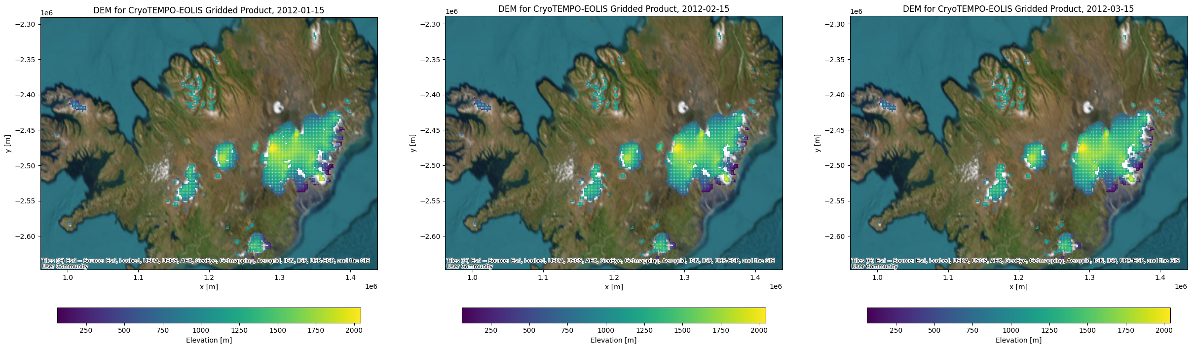
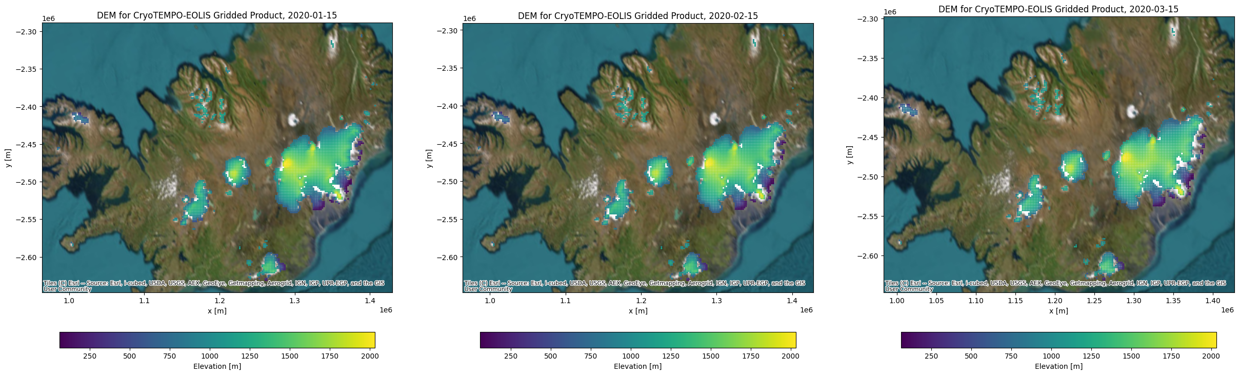
We see that, in the Iceland region, the Gridded Product has particularly good coverage over Vatnajökull ice cap.

Plot elevation difference

Let’s plot the elevation difference between January 2012 and January 2020 data to investigate further.

jan_2012_source_id = gridded_product_data_2012.iloc[0]['source_id']
jan_2020_source_id = gridded_product_data_2020.iloc[0]['source_id']

jan_2012_data = gridded_product_data_2012[gridded_product_data_2012['source_id']
                                          == jan_2012_source_id]
jan_2020_data = gridded_product_data_2020[gridded_product_data_2020['source_id']
                                          == jan_2020_source_id]

merged_gdf = jan_2012_data.sjoin(df=jan_2020_data, how='inner')
merged_gdf['elevation_difference'] = merged_gdf['elevation_right'] - \
    merged_gdf['elevation_left']

ax = merged_gdf.to_crs(epsg=3413).plot(column=merged_gdf['elevation_difference'], figsize=(
    10, 10), legend=True, cmap='magma_r', s=3, legend_kwds={
        'label': 'Elevation change [m]', 'orientation': 'horizontal'
    })
ax.set_xlabel('x [m]')
ax.set_ylabel('y [m]')
ax.set_title(f"Elevation difference between Jan 2012 and Jan 2020 in Iceland")
ctx.add_basemap(ax, source=ctx.providers.GeoportailFrance.orthos, crs=3413, zoom=8)

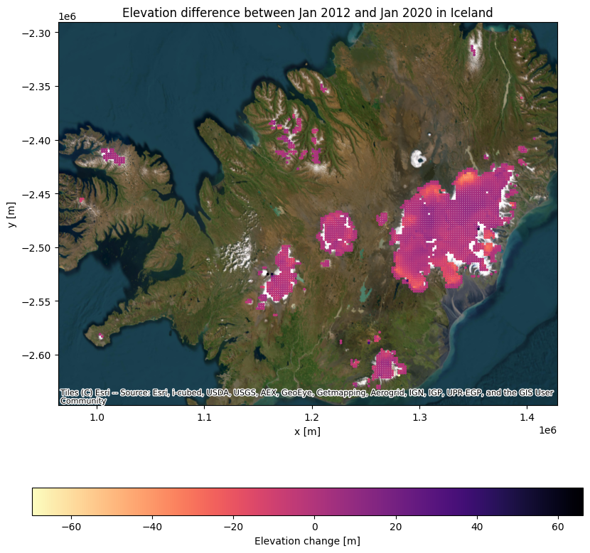
The above shows a significant decrease of ice elevation in the glacier margins at low elevations, this is particularly visible in Vatnajökull ice cap.