CryoTEMPO-EOLIS Gridded Product & RGI: Comparing Elevation Changes of Surging and Non-Surging Glaciers in Svalbard

Introduction

This example retrieves CryoTEMPO-EOLIS Gridded Product data over 12 years using the RGI v7.0 glacier boundary definitions, and analyses the elevation changes for different surge-type glaciers across Svalbard.

For details on environment and Specklia client setup, please see Environment Setup.

Query RGI polygons

Firstly, let’s use Specklia to retrieve the RGI polygons for glaciers in Svalbard.

svalbard_polygon = shapely.Polygon(([3.9, 79.88], [28.6, 80.97], [28.6, 77.03], [14.57, 75.51], [3.9, 79.88]))

available_datasets = client.list_datasets()
rgiv7_dataset = available_datasets[available_datasets['dataset_name'] == 'RGIv7 Glaciers'].iloc[0]
rgi_data, rgi_data_sources = client.query_dataset(
    dataset_id=rgiv7_dataset['dataset_id'],
    epsg4326_polygon=svalbard_polygon,
    min_datetime=rgiv7_dataset['min_timestamp'] - Timedelta(seconds=1),
    max_datetime=rgiv7_dataset['max_timestamp'] + Timedelta(seconds=1))

The RGI dataset provides a surge_type attribute categorising each glacier based on evidence of surging. Surging is typically short-lived events where a glacier moves many times its normal rate.

From the RGI v7.0 user guide we get the surge_type definitions:

surge_type_definitions = {0: 'No evidence', 1: 'Possible', 2: 'Probable', 3: 'Observed', 9: 'Not assigned'}

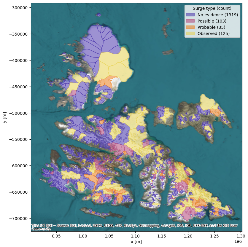
We can now plot the glacier boundaries on a map and colour code them by surge-type to see where they are.

fig, ax = plt.subplots(figsize=(10, 10))
legend_elements = []
glacier_polygons = {}
for i, (surge_id, surge_type) in enumerate(surge_type_definitions.items()):
    # we use a simplified version of the RGI polygons, which has a reduced number of vertices
    polygons_for_surge_type = gpd.GeoSeries(
        rgi_data[rgi_data.surge_type == surge_id]['simplified_polygons_t200'], crs=rgi_data.crs)

    if not polygons_for_surge_type.empty:
        glacier_polygons[surge_type] = polygons_for_surge_type

        color = cm.CMRmap((i + 1) / (len(surge_type_definitions)))
        polygons_for_surge_type.to_crs(nps_epsg_code).plot(ax=ax, facecolor=color, edgecolor=color, alpha=0.5)
        legend_elements.append(Patch(facecolor=color, edgecolor=color,
                                    label=surge_type + f' ({len(polygons_for_surge_type)})',
                                    alpha=0.5))
ax.set_xlabel('x [m]')
ax.set_ylabel('y [m]')
ax.legend(handles=legend_elements, loc='upper right', title='Surge type (count)')
ctx.add_basemap(ax, source=ctx.providers.GeoportailFrance.orthos, crs=nps_epsg_code, zoom=6)
plt.show()

Query data for each surge-type category

Now that we have the glacier boundary definitions for each surge-type we can query the CryoTEMPO-EOLIS gridded dataset.

svalbard_eolis_data = {}
svalbard_data_sources = {}

dataset_name = 'CryoTEMPO-EOLIS Gridded Product'
gridded_product_dataset = available_datasets[
    available_datasets['dataset_name'] == dataset_name].iloc[0]

for surge_id, surge_type in surge_type_definitions.items():
    if surge_type not in glacier_polygons:
        print(f'No data to query as there are no glaciers of surge type: {surge_type}, skipping..')
        continue
    query_polygon = glacier_polygons[surge_type].unary_union

    query_start_time = perf_counter()
    svalbard_eolis_data[surge_type], svalbard_data_sources[surge_type] = client.query_dataset(
        dataset_id=gridded_product_dataset['dataset_id'],
        epsg4326_polygon=query_polygon,
        min_datetime=datetime(2011, 1, 1),
        max_datetime=datetime(2023, 11, 1),
        columns_to_return=['timestamp', 'elevation', 'uncertainty'])

    print(f'Query of glaciers of surge type: {surge_type} complete in '
          f'{perf_counter()-query_start_time:.2f} seconds, '
          f'{len(svalbard_eolis_data[surge_type])} points returned, '
          f'drawn from {len(svalbard_data_sources[surge_type])} original sources.')

Query of glaciers of surge type: No evidence complete in 16.09 seconds, 528076 points returned, drawn from 154 original sources.
Query of glaciers of surge type: Possible complete in 5.47 seconds, 84104 points returned, drawn from 154 original sources.
Query of glaciers of surge type: Probable complete in 5.89 seconds, 75051 points returned, drawn from 154 original sources.
Query of glaciers of surge type: Observed complete in 8.31 seconds, 417317 points returned, drawn from 154 original sources.
No data to query as there are no glaciers of surge type: Not assigned, skipping..

Compare elevation change time series per surge-type

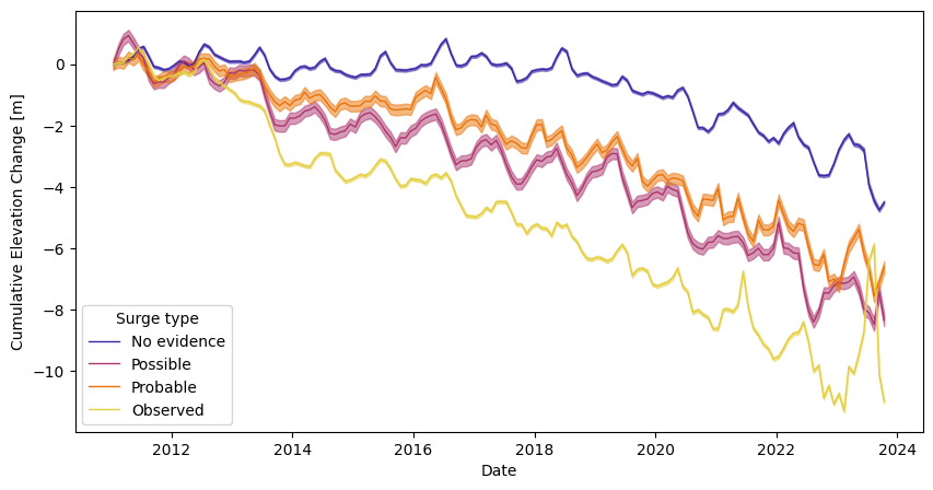
From the Gridded Product documentation, we know that it is generated at a monthly temporal resolution.

We can now construct a monthly cumulative elevation change timeseries for glaciers of each surge-type.

def calculate_time_series(gridded_product_data: gpd.GeoDataFrame) -> Tuple[NDArray, NDArray, List[int]]:
    """
    Calculate a weighted average elevation change per month and associated errors.

    Weights are assigned using the CryoTEMPO-EOLIS gridded product uncertainty.

    Parameters
    ----------
    gridded_product_data : gpd.GeoDataFrame
        CryoTEMPO-EOLIS gridded product data.

    Returns
    -------
    Tuple[NDArray, NDArray, List[int]]
        Weighted average elevation change elevation change per month, error on weighted average,
        and dates of each timestep.
    """
    unique_timestamps = sorted(gridded_product_data.timestamp.unique())

    # elevation change is in reference to first gridded product
    reference_dem = gridded_product_data[gridded_product_data.timestamp == unique_timestamps[0]]

    # initialise empty lists for time series data
    weighted_mean_timeseries = []
    weighted_mean_errors = []
    for unique_timestamp in unique_timestamps:
        gridded_product_for_timestamp = gridded_product_data[gridded_product_data.timestamp == unique_timestamp]
        merged_gdf = reference_dem.sjoin(df=gridded_product_for_timestamp, how='inner')
        merged_gdf['elevation_difference'] = merged_gdf['elevation_right'] - merged_gdf['elevation_left']

        # combine uncertainties for elevation difference
        merged_gdf['elevation_difference_unc'] = np.sqrt(
            merged_gdf['uncertainty_right']**2 + merged_gdf['uncertainty_left']**2)

        # calculate average elevation change, weighted by measurement uncertainty
        weighted_mean = (np.sum(merged_gdf['elevation_difference'] / merged_gdf['elevation_difference_unc']**2)
                        / np.sum(1 / merged_gdf['elevation_difference_unc']**2))

        # calculate weighted average uncertainty
        error = np.sqrt(1 / np.sum(1 / merged_gdf['elevation_difference_unc']**2))

        weighted_mean_timeseries.append(weighted_mean)
        weighted_mean_errors.append(error)

    dates = [datetime.fromtimestamp(ts) for ts in unique_timestamps]

    return np.array(weighted_mean_timeseries), np.array(weighted_mean_errors), dates

Plotting this time series, we see how the glaciers that are known to surge, or possible surging glaciers, are reducing in elevation more than non-surging glaciers.

fig, ax = plt.subplots(figsize=(10, 5))

for i, (surge_type, gridded_product_data) in enumerate(svalbard_eolis_data.items()):
    # calculate time series for surge type
    weighted_mean_timeseries, weighted_mean_errors, dates = calculate_time_series(gridded_product_data)

    # plot time series
    color = cm.CMRmap((i + 1) / (len(surge_type_definitions)))
    ax.plot(dates, weighted_mean_timeseries, lw=1, label=surge_type, c=color)
    ax.fill_between(dates,
                     weighted_mean_timeseries - weighted_mean_errors,
                     weighted_mean_timeseries + weighted_mean_errors,
                     alpha=0.5,
                     color=color)

ax.set_xlabel('Date')
ax.set_ylabel('Cumulative Elevation Change [m]')
ax.legend(title='Surge type')
plt.show()

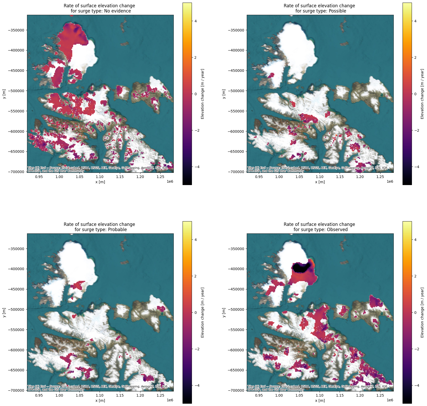
Map rate of surface elevation change

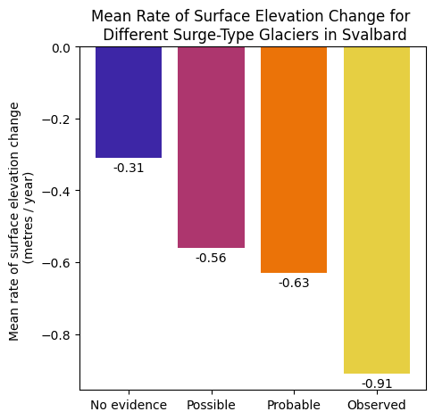
Finally, we can calculate the rate of surface elevation change per year by applying a least squares regression to all data points for each pixel.

We can plot this spatially for the different surge-types to see how the glacier elevation is changing across svalbard, and plot the mean rate of elevation change per surge-type.

def calculate_rate_of_change_map(gridded_product_data: gpd.GeoDataFrame) -> gpd.GeoDataFrame:
    """
    Apply least squares linear regression to each pixel through time.

    Parameters
    ----------
    gridded_product_data : gpd.GeoDataFrame
        CryoTEMPO-EOLIS gridded product data.

    Returns
    -------
    gpd.GeoDataFrame
        Rate of surface elevation change per year per pixel.
    """
    pixel_groups = gridded_product_data.groupby(by='geometry')
    rate_of_surface_elevation_change_years = []
    for _, pixel_group in pixel_groups:
        pixel_group_df = pixel_group.sort_values(by='timestamp')
        m, _ = np.linalg.lstsq(
            np.vstack([pixel_group_df['timestamp'].to_numpy(), np.ones(len(pixel_group_df))]).T,
            pixel_group_df.elevation.to_numpy(),
            rcond=None)[0]
        # m gives the rate of change of elevation in seconds, lets crudely convert it to years for a more meaningful value
        rate_of_surface_elevation_change_years.append(m * 60 * 60 * 24 * 365)
    dhdt_gdf = gpd.GeoDataFrame({'rate_of_surface_elevation_change_years': rate_of_surface_elevation_change_years},
                                geometry=[key for key, _ in pixel_groups], crs=gridded_product_data.crs)
    return dhdt_gdf

fig, axes = plt.subplots(figsize=(20, 20), nrows=2, ncols=2)
axes = axes.flatten()

min_x, min_y, max_x, max_y = rgi_data.to_crs(nps_epsg_code).total_bounds

mean_rate_of_change_for_surge_types = []
for i, (surge_type, gridded_product_data) in enumerate(svalbard_eolis_data.items()):
    # calculate rate of surface elevation change for pixel over time
    dhdt_gdf = calculate_rate_of_change_map(gridded_product_data)
    mean_rate_of_change_for_surge_types.append(dhdt_gdf['rate_of_surface_elevation_change_years'].mean())

    # plot rate of surface elevation change on map
    dhdt_gdf.to_crs(epsg=nps_epsg_code).plot(
        ax=axes[i], column='rate_of_surface_elevation_change_years', s=5, cmap='inferno', vmin=-5, vmax=5,
        legend=True, legend_kwds={"label": "Elevation change [m / year]"})

    axes[i].set_xlim(min_x, max_x)
    axes[i].set_ylim(min_y, max_y)
    axes[i].set_xlabel('x [m]')
    axes[i].set_ylabel('y [m]')
    axes[i].set_title(f'Rate of surface elevation change \n for surge type: {surge_type}')

    ctx.add_basemap(axes[i], source=ctx.providers.GeoportailFrance.orthos, crs=nps_epsg_code, zoom=6)
plt.show()

fig, ax = plt.subplots(figsize=(5, 5))
# round mean rate of change to 2 decimal places
rects = ax.bar(svalbard_eolis_data.keys(), [round(mean_rate, 2) for mean_rate in mean_rate_of_change_for_surge_types],
        color=[cm.CMRmap((i + 1) / (len(surge_type_definitions))) for i in range(len(svalbard_eolis_data))])
ax.bar_label(rects, padding=3)
plt.ylabel('Mean rate of surface elevation change \n (metres / year)')
plt.title('Mean Rate of Surface Elevation Change for \n Different Surge-Type Glaciers in Svalbard')
plt.show()