CryoTEMPO-EOLIS Point product - quality and coverage

This example investigates the coverage and quality of the CryoTEMPO-EOLIS Point Product while using Specklia to retrieve the data.

For details on environment and Specklia client setup, please see to Environment Setup.

Explore dataset source files

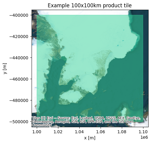
The CryoTEMPO-EOLIS Point Product documentation tells us that it is generated at a monthly temporal resolution, one product file per 100x100km tile.

Let’s run a small query and use the returned source files to determine the bounding polygon of an example tile.

svalbard_polygon = shapely.Polygon(([3.9, 79.88], [34.64, 80.97], [
    36.86, 77.03], [14.57, 75.51], [3.9, 79.88]))

dataset_name = 'CryoTEMPO-EOLIS Point Product'
available_datasets = client.list_datasets()
point_product_dataset = available_datasets[
    available_datasets['dataset_name'] == dataset_name].iloc[0]

point_product_data, sources = client.query_dataset(
    dataset_id=point_product_dataset['dataset_id'],
    epsg4326_polygon=svalbard_polygon,
    min_datetime=datetime.datetime(2023, 1, 1),
    max_datetime=datetime.datetime(2023, 1, 2),
    columns_to_return=['timestamp', 'elevation', 'uncertainty'])

print(
    f'Query complete, {len(point_product_data)} points returned, drawn from {len(sources)} original sources.')

Query complete, 98044 points returned, drawn from 4 original sources.

We pick a source at random, and retrieve its geospatial bounding box.

source_info = sources[1]['source_information']

tile_x_min = source_info['geospatial_x_min']
tile_x_max = source_info['geospatial_x_max']
tile_y_min = source_info['geospatial_y_min']
tile_y_max = source_info['geospatial_y_max']

tile_polygon_points = [(tile_x_min, tile_y_min), (tile_x_min, tile_y_max),
                       (tile_x_max, tile_y_max), (tile_x_max, tile_y_min)]

We must query Specklia with a polygon in the EPSG4326 projection, so let’s transform the information we have just retrieved and plot it.

source_projection = pyproj.CRS.from_proj4(source_info['geospatial_projection'])
desired_projection = pyproj.CRS.from_epsg('4326')
transformer = pyproj.Transformer.from_proj(
    source_projection, desired_projection, always_xy=True)

tile_polygon = shapely.Polygon([transformer.transform(p[0], p[1])
                                for p in tile_polygon_points])

tile_spatial_coverage = gpd.GeoDataFrame(
    geometry=[tile_polygon], crs=4326)

ax = tile_spatial_coverage.to_crs(epsg=3413).plot(
    figsize=(5, 5), alpha=0.5, color=data_coverage_color, edgecolor=data_coverage_color)
ax.set_xlabel('x [m]')
ax.set_ylabel('y [m]')
ax.set_title(f"Example 100x100km product tile")
ctx.add_basemap(ax, source=ctx.providers.GeoportailFrance.orthos, crs=3413, zoom=8)

Query dataset

Now that we have the bounding box of our 100x100km tile, let’s use it for a query.

According to the definition of the point product, querying the dataset over a single tile over a time window of 3 months should return data from 3 original sources. Let’s check.

point_product_data, sources = client.query_dataset(
    dataset_id=point_product_dataset['dataset_id'],
    epsg4326_polygon=tile_polygon,
    min_datetime=datetime.datetime(2023, 1, 1),
    max_datetime=datetime.datetime(2023, 3, 31),
    columns_to_return=['timestamp', 'elevation', 'uncertainty', 'x', 'y'])

print(
    f'Query complete, {len(point_product_data)} points returned, drawn from {len(sources)} original sources.')

Query complete, 1335027 points returned, drawn from 3 original sources.

Plot coverage

Now, let’s plot the data coverage.

from mpl_toolkits.axes_grid1 import make_axes_locatable

fig, axs = plt.subplots(1, 2, figsize=(20, 10), sharex=True)
point_product_data.dropna(inplace=True)
point_product_data_3413 = point_product_data.to_crs(epsg=3413)
divider = make_axes_locatable(axs[0])
cax = divider.append_axes("right", size="5%", pad=0.1)
point_product_data_3413.plot(
    ax=axs[0], column=point_product_data['elevation'], s=1, cmap='viridis', legend=True, legend_kwds={
        "cax": cax,
        "label": "Elevation [m]"
    }, )

axs[0].set_xlabel('x [m]')
axs[0].set_ylabel('y [m]')

divider = make_axes_locatable(axs[1])
cax = divider.append_axes("right", size="5%", pad=0.1)
point_product_data_3413.plot(
    ax=axs[1], column=point_product_data['uncertainty'], s=1, cmap='viridis', legend=True, legend_kwds={
        "cax": cax,
        "label": "Uncertainty [m]"
    })
axs[1].set_xlabel('x [m]')

plt.ticklabel_format(axis='x', style='sci', scilimits=(0, 0))
t = plt.suptitle(
    'Coverage of CryoTEMPO-EOLIS point product over example 100x100km tile')
ctx.add_basemap(axs[0], source=ctx.providers.GeoportailFrance.orthos, crs=3413, zoom=8)
ctx.add_basemap(axs[1], source=ctx.providers.GeoportailFrance.orthos, crs=3413, zoom=8)

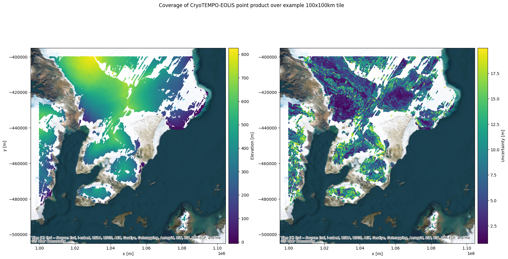
The plot shows all point data available in our 100x100km tile in the timeframe that we specified for the query, and demonstrates the spatial coverage achieved using swath processing.

In the figure on the left, the scatter points are colour-coded by their elevations. On the right, the colour shows the uncertainty associated with each point.

For more information on CryoSat-2 and swath processing, see https://earth.esa.int/eogateway/news/cryosats-swath-processing-technique.

Explore data quality

Firstly we calculate the mean and median uncertainties, as well as the standard deviation.

med_unc = np.nanmedian(point_product_data['uncertainty'])
mean_unc = np.nanmean(point_product_data['uncertainty'])
std_unc = np.std(point_product_data['uncertainty'])

We next set up some histogram bins, requiring 40 bins in the uncertainty range.

bins = np.linspace(np.nanmin(point_product_data['uncertainty']), np.nanmax(
    point_product_data['uncertainty']), 40)

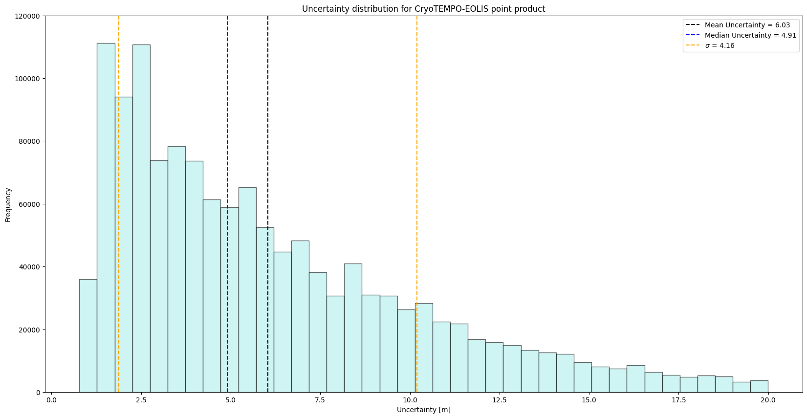
Finally, we plot a histogram of the uncertainty values for this point product dataset, and display the mean and median values, as well as the standard deviation of uncertainties.

fig, axs = plt.subplots(1, 1, figsize=(20, 10))

a = axs.hist(point_product_data['uncertainty'], bins=bins,
             facecolor='paleturquoise', edgecolor='k', alpha=0.6)

axs.vlines(mean_unc, 0, 12e4, color='k', linestyle='dashed',
           label='Mean Uncertainty = {:0.2f}'.format(mean_unc))
axs.vlines(med_unc, 0, 12e4, color='b', linestyle='dashed',
           label='Median Uncertainty = {:0.2f}'.format(med_unc))
axs.vlines(mean_unc - std_unc, 0, 12e4, color='orange', linestyle='dashed')
axs.vlines(mean_unc + std_unc, 0, 12e4, color='orange',
           linestyle='dashed', label='$\sigma$ = {:0.2f}'.format(std_unc))

axs.set_ylim(0, 12e4)
axs.set_xlabel('Uncertainty [m]')
axs.set_ylabel('Frequency')
axs.set_title('Uncertainty distribution for CryoTEMPO-EOLIS point product')
plt.legend()

<matplotlib.legend.Legend at 0x7f8dc1b64700>